OS 调度器
Dec 9, 2020 21:30 · 7288 words · 15 minute read

译文
介绍
Go 调度器的设计能够使得你的多线程 Go 程序更高效、性能更好,得益于 Go 调度器对操作系统调度器的合理利用。但如果你的多线程 Go 程序写得很烂,那还是白搭。大概了解操作系统和 Go 调度器的工作原理对正确地设计多线程的程序很有帮助。
本文将着重于更高层次的调度器机制和语义,提供足够多的细节来让你能够直观地了解其工作原理,从而做出更好的工程决策。尽管还有更多方面需要斟酌,但这部分基础知识还是要知道的。
OS 调度器
操作系统调度器非常复杂,必须考虑到硬件,包括但不限于存在多个处理器与核心,CPU 缓存与 NUMA。没有这些知识,调度器无法做到尽可能的高效。幸运的是,你仍然可以在不深入研究这些话题的情况下,较好地理解操作系统调度器的工作方式。
你的程序就是一串机器指令,一条接一条地顺序执行。为了实现这个,操作系统使用了“线程”概念。线程的工作是执行分配给它的指令集,直到没有指令可执行为止。
每个程序都会创建一个进程,每个进程都是一个初始的线程,线程能够衍生更多线程。所有这些不同的线程都相互独立运行,调度决策是线程级的而不是进程级的。线程可以并发运行(每个都占用独立的 CPU 核心一段时间片),或者并行(同时在不同的核心跑)。为了安全、局部、独立地执行自己的指令,线程会维护它们自己的状态。
操作系统调度器的工作就是,只要有线程可以被执行时那 CPU 核心尽量不被闲置。它也创造了线程同时在执行的假象。在制造这个假象时,调度器需要运行优先级较高的线程而不是低优先级的线程。但是呢,低优先级的线程也不能长期处于“饥饿”状态。调度器本身也要尽可能最小化调度延迟以做出更快更聪明的决策。
为了实现这些要搞一堆算法,但幸运的是行业已经有几十年的经验了。为了更好地理解这些,最好先讲一些概念。
执行指令
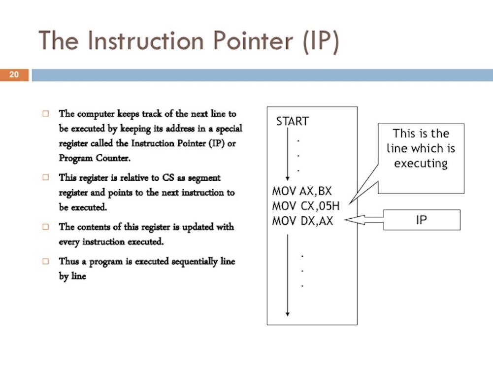
程序计数器(PC),有时候被称作指令指针(IP),线程用它来追踪下一步要执行的指令。大多数处理器 PC 指向下一条指令而不是当前指令。
如果你看过 Go 程序的栈,可能会注意到每行末尾的十六进制数字:
goroutine 1 [running]:
   main.example(0xc000042748, 0x2, 0x4, 0x106abae, 0x5, 0xa)
       stack_trace/example1/example1.go:13 +0x39                 <- LOOK HERE
   main.main()
       stack_trace/example1/example1.go:8 +0x72                  <- LOOK HERE
这些数字表示 PC 距离各自函数栈顶的偏移量。PC 的偏移量为 +0x39 表示线程在 example 函数中将要执行的下一条指令;PC 的偏移量为 0+x72 则是 main 函数中下一条指令(如果回得去的话)。更重要的是,PC 之前的指令告诉了你正在执行什么东西。
上述的栈来自于下面的代码 https://github.com/ardanlabs/gotraining/blob/master/topics/go/profiling/stack_trace/example1/example1.go:
func main() {
    example(make([]string, 2, 4), "hello", 10)
}

func example(slice []string, str string, i int) {
   panic("Want stack trace")
}
+0x39 表示自 example 函数开始的地方往下 57 字节。将二进制反汇编,找到第 12 条指令,在最底部:
$ go tool objdump -S -s "main.example" ./example1
TEXT main.example(SB) stack_trace/example1/example1.go
func example(slice []string, str string, i int) {
  0x104dfa0		65488b0c2530000000	MOVQ GS:0x30, CX
  0x104dfa9		483b6110		CMPQ 0x10(CX), SP
  0x104dfad		762c			JBE 0x104dfdb
  0x104dfaf		4883ec18		SUBQ $0x18, SP
  0x104dfb3		48896c2410		MOVQ BP, 0x10(SP)
  0x104dfb8		488d6c2410		LEAQ 0x10(SP), BP
	panic("Want stack trace")
  0x104dfbd		488d059ca20000	LEAQ runtime.types+41504(SB), AX
  0x104dfc4		48890424		MOVQ AX, 0(SP)
  0x104dfc8		488d05a1870200	LEAQ main.statictmp_0(SB), AX
  0x104dfcf		4889442408		MOVQ AX, 0x8(SP)
  0x104dfd4		e8c735fdff		CALL runtime.gopanic(SB)
  0x104dfd9		0f0b			UD2              <--- LOOK HERE PC(+0x39)
上面的那行指令引发了 panic。
PC 是下一条指令,不是当前的。
线程状态
另一个重要概念是线程状态,有三种:等待、可运行和执行中。
等待:线程已经停止并在等待(比如 I/O,系统调用或者同步调用)完成才能继续。这是导致性能瓶颈的万恶之源。 可运行:线程想要一段时间片来执行分配好的机器指令。如果有很多这样的线程,那就得等更久了。此外由于更多的线程争抢时间片,每条线程分到的时间就更短了。这种调度延迟也会导致差劲的性能。 正在执行:线程已经分到了核心并且正在执行指令。与应用程序相关的工作已经完成,这是皆大欢喜。
任务种类
CPU 密集型:线程从不处于等待状态,就不停地计算。一个正在运行计算 π 到 N 位的线程就是 CPU 密集型。 IO 密集型:这种任务会导致线程进入等待状态,比如网络请求或系统调用。一个要访问数据库的线程也是 IO 密集型,我会把导致线程等待的同步事件(互斥锁、原子操作)也归类到这。
上下文切换
Linux、MacOS 和 Windows 都是抢占式调度器。也就是说调度器是不可预测的,线程的优先级和事件(比如网络接收数据)使我们无法确定调度器的选择。千万不要带着侥幸心理编码,已经发生过 1000 次不代表每一次都发生。如果你要应用程序是确定的,那就必须控制线程的同步和协调。
CPU 核心上线程切换的操作被叫做上下文切换。当调度器将一个正在执行的线程从核心抽出,并将其替换为一个可运行的线程时,就会发生上下文切换。运行队列中被选中的线程会进入正在执行状态,放回去的线程被改回可运行状态或者进入等待状态(因为 IO 类型的请求被切换)。
上下文切换开销很大因为要把线程切入切出 CPU 核心很费时间,延迟视情况而定,从 1000 到 1500 纳秒不等。考虑到硬件平均每个核心每纳秒要执行 12 条指令,一次上线切换会耗费 12000 到 18000 条指令的延迟,实质上你的程序在上下文切换期间失去了执行大量指令的能力。
如果你的程序是 IO 密集型的,那上下文切换是家常便饭。每当有线程变成等待状态,另外一个可运行的线程会取代它的位置,使得 CPU 核心是一直在作业的,这是调度的核心原则,还有任务未完成就不能让 CPU 闲着。
如果你的程序是 CPU 密集型的,上下文切换则是性能噩梦。由于线程总是有作业,上下文切换阻止了工作的进展。这种情况与 IO 密集型的工作负载形成了鲜明的对比。
少即是多
早期的处理器只有单核,调度还没那么复杂。单处理器单核在任何给定的时间只能执行一个线程。我们的想法是定义一个调度周期,并尝试在这段时间内执行所有可运行的线程。没有问题:把调度周期除以需要执行的线程数量。
举个栗子,如果把调度周期定义成 1000ms(也就是1 秒)并且有十个线程,那么每个线程分到 100ms。如果有一百个线程,每个线程就分到 10ms。但是,当有一千个线程时会发生啥?给每个线程 1ms 的时间片是行不通的,因为花在上下文切换的时间比例和花在作业上的时间有很大关系。
你需要对给定的时间片做一个小限制。在上面的场景中,如果最小的时间片是 10ms,而你有一千个线程,那么调度周期需要增加到 10000ms(10 秒);如果有一万个线程,现在的调度周期是 100000ms 了。在一万个线程的情况下,最小时间片是 10ms,如果每个线程都用尽了它们的时间片,那么所有的线程都运行一把要 100 秒。
在做调度决策时,调度器要考虑和处理很多的东西。你可以控制你应用程序中使用线程的数量(线程池技术)。当线程越来越多,并且还是 IO 密集型的作业,就会变得越来越混乱和不确定,调度和执行需要更多的时间。
这就是为什么这个游戏规则是“少即是多”。可运行状态的线程越少,意味着调度开销越少,每个线程获得的时间就更多。更多处于可运行状态的线程也就意味着随着时间的流逝所获得的的时间越少,作业时间也就少了。
寻求平衡
要在 CPU 核心数量和线程数量之间找到平衡点来为应用程序获得最佳吞吐量,线程池是一个很棒的答案。写 Go 程序就没必要这么搞了,我认为 Go 让多线程应用程序开发更容易了。
在 Go 之前我用 C++ 和 C# 面向 NT 内核编程,在那个操作系统上,IOCP 线程池的使用对多线程软件的编写是至关重要的。作为一个工程师,你得算清楚需要多少线程池以及每个池的最大线程数量,在给定核心数量下最大化吞吐量。
当开发与数据库通讯的 web 服务时,每核 3 线程这个魔法量看上去总是能在 NT 内核上提供最好的吞吐量。换句话说,每核 3 线程最大程度地降低了上下文切换的延迟成本,同时最大化了核心的执行时间。如果我每核使用两个线程,就要更长的时间来完成所有工作,因为有部分时间核心是闲置的,它本该处于工作状态;如果我每核使用 4 个线程,也要更长的时间,因为上下文切换造成了更多的延迟。每个核心 3 线程似乎总是 NT 内核上的魔法数字。
要是你的服务正在混合作业,可能会产生不同且不一致的延迟,甚至还会搞出不少系统级的事件。弄不好就找不到这样一个对不同工作负载都有效的魔法数字。当涉及到使用线程池来对性能调优,要找到正确的配置可能相当麻烦。
多级缓存
从主存访问数据开销相当大(100 到 300 个时钟周期),而从缓存访问数据开销小多了(3 到 40 个时钟周期)。现在要编写高性能的多线程应用程序,一方面是关于如何高效地将数据送入处理器,还要考虑缓存系统的机制。
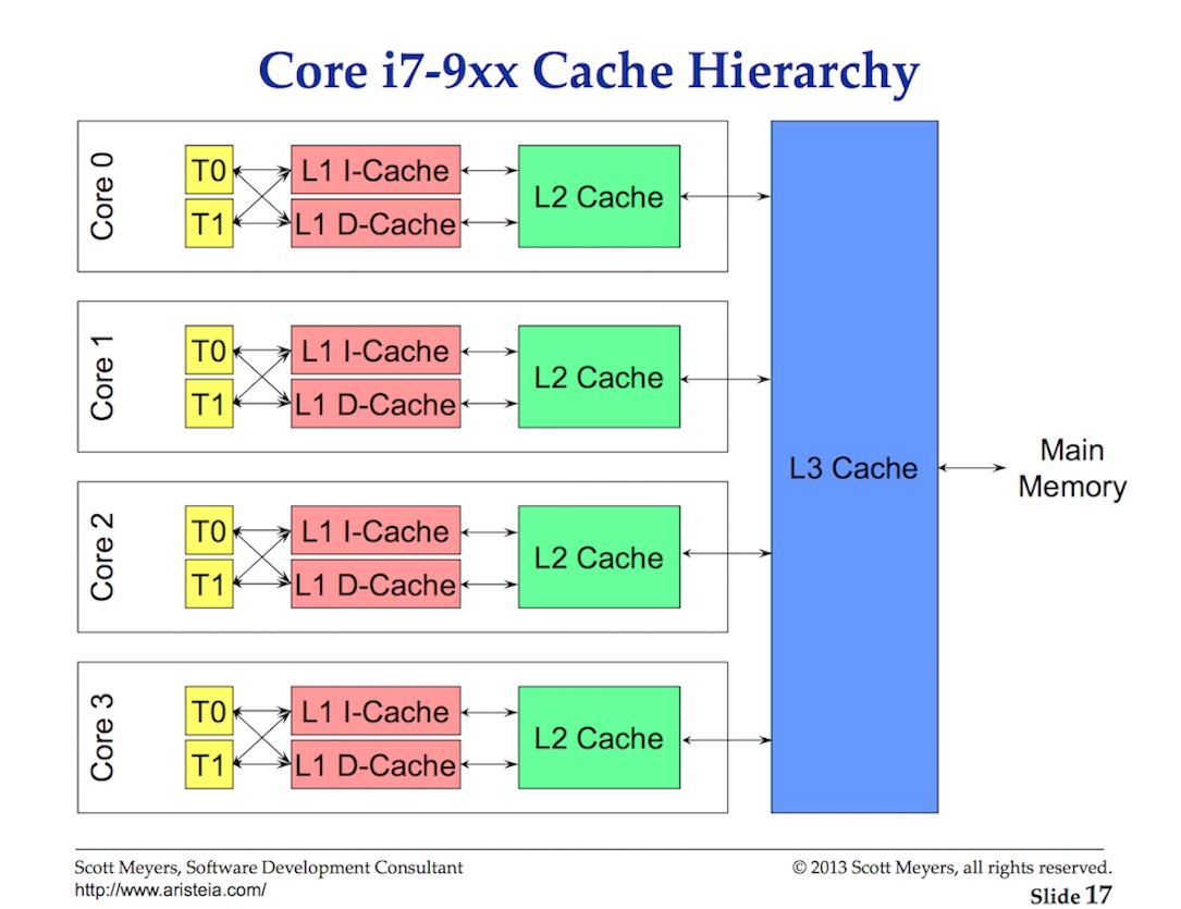
处理器使用多级缓存与主存交换数据,是一段 64 字节的存储块。每个核心会分到它需要的缓存流水线的副本,也就是说硬件使用值语义。这也是为什么内存的突变是多线程应用程序的性能噩梦。
当多条线程访问同一个数据,它们将先在同一个缓存上访问。在任何核心上运行的任何线程都会得到自己的同一条缓存流水线的副本。
如果某个线程更改了它的缓存,那么通过硬件的能力,所有其他副本都必须被标记为 dirty。当一个线程试图访问被“污染”的缓存,需要访问主存(100 到 300 个时钟周期)才能得到新的缓存副本。
也许在双核处理器上这还是小意思,但 32 核处理器并行跑着 32 个线程,而所有线程都在同一条缓存流水线上读写数据呢?如果系统有两个处理器呢?这就更糟了,因为处理器和处理器直接的通讯还增大了延迟。应用程序在内存中大打出手,而且查都没法查。
这被称为缓存一致性问题,在编写多线程应用程序时要考虑的。
调度决策场景
启动一个应用程序,主线程在 1 号核心上执行。当线程开始执行指令时,缓存也正被检索。现在线程要创建一个新的线程做些并发处理。那么问题来了:
- 将主线程切换出 1 号 CPU 核心?这样可以提高性能,因为缓存大概率有它想要的数据。但是主线程就得不到完整的时间片了。
- 在主线程的时间片用完前,要不要等核心 1 腾出来,线程只要一启动就跑的飞快因为少了取数据的延迟。
- 线程要等待下一个可用的核心吗?这意味着所选核心的缓存将被刷新造成延迟。但是线程将更快地启动而且主线程的时间片是完整的。
有意思吗?这些都是 OS 调度器在决策前要考虑的。万幸,我不是干这行的,我可以告诉大家的也就是,如果核心闲置了,要把它利用起来。你要让线程尽可能运行起来。
总结
这个系列的第一部分将深入介绍在编写多线程应用程序时必须考虑的线程和操作系统调度器的那些事。这也是 Go 调度器要考虑的。下一篇我会讲述 Go 调度器的语义,还有它是如何与这些概念关联的。
原文
Introduction
The design and behavior of the Go scheduler allows your multithreaded Go programs to be more efficient and performant. This is thanks to the mechanical sympathies the Go scheduler has for the operating system (OS) scheduler. However, if the design and behavior of your multithreaded Go software is not mechanically sympathetic with how the schedulers work, none of this will matter. It’s important to have a general and representative understanding of how both the OS and Go schedulers work to design your multithreaded software correctly.
This multi-part article will focus on the higher-level mechanics and semantics of the schedulers. I will provide enough details to allow you to visualize how things work so you can make better engineering decisions. Even though there is a lot that goes into the engineering decisions you need to make for multithreaded applications, the mechanics and semantics form a critical part of the foundational knowledge you need.
OS Scheduler
Operating-system schedulers are complex pieces of software. They have to take into account the layout and setup of the hardware they run on. This includes but is not limited to the existence of multiple processors and cores, CPU caches and NUMA. Without this knowledge, the scheduler can’t be as efficient as possible. What’s great is you can still develop a good mental model of how the OS scheduler works without going deep into these topics.
Your program is just a series of machine instructions that need to be executed one after the other sequentially. To make that happen, the operating system uses the concept of a Thread. It’s the job of the Thread to account for and sequentially execute the set of instructions it’s assigned. Execution continues until there are no more instructions for the Thread to execute. This is why I call a Thread, “a path of execution”.
Every program you run creates a Process and each Process is given an initial Thread. Threads have the ability to create more Threads. All these different Threads run independently of each other and scheduling decisions are made at the Thread level, not at the Process level. Threads can run concurrently (each taking a turn on an individual core), or in parallel (each running at the same time on different cores). Threads also maintain their own state to allow for the safe, local, and independent execution of their instructions.
The OS scheduler is responsible for making sure cores are not idle if there are Threads that can be executing. It must also create the illusion that all the Threads that can execute are executing at the same time. In the process of creating this illusion, the scheduler needs to run Threads with a higher priority over lower priority Threads. However, Threads with a lower priority can’t be starved of execution time. The scheduler also needs to minimize scheduling latencies as much as possible by making quick and smart decisions.
A lot goes into the algorithms to make this happen, but luckily there are decades of work and experience the industry is able to leverage. To understand all of this better, it’s good to describe and define a few concepts that are important.
Executing Instructions
The program counter (PC), which is sometimes called the instruction pointer (IP), is what allows the Thread to keep track of the next instruction to execute. In most processors, the PC points to the next instruction and not the current instruction.
If you have ever seen a stack trace from a Go program, you might have noticed these small hexadecimal numbers at the end of each line. Look for +0x39 and +0x72 in Listing 1.
goroutine 1 [running]:
   main.example(0xc000042748, 0x2, 0x4, 0x106abae, 0x5, 0xa)
       stack_trace/example1/example1.go:13 +0x39                 <- LOOK HERE
   main.main()
       stack_trace/example1/example1.go:8 +0x72                  <- LOOK HERE
Those numbers represent the PC value offset from the top of the respective function. The +0x39 PC offset value represents the next instruction the Thread would have executed inside the example function if the program hadn’t panicked. The 0+x72 PC offset value is the next instruction inside the main function if control happened to go back to that function. More important, the instruction prior to that pointer tells you what instruction was executing.
Look at the program below in Listing 2 which caused the stack trace from Listing 1. https://github.com/ardanlabs/gotraining/blob/master/topics/go/profiling/stack_trace/example1/example1.go
func main() {
    example(make([]string, 2, 4), "hello", 10)
}

func example(slice []string, str string, i int) {
   panic("Want stack trace")
}
The hex number +0x39 represents the PC offset for an instruction inside the example function which is 57 (base 10) bytes below the starting instruction for the function. In Listing 3 below, you can see an objdump of the example function from the binary. Find the 12th instruction, which is listed at the bottom. Notice the line of code above that instruction is the call to panic.
$ go tool objdump -S -s "main.example" ./example1
TEXT main.example(SB) stack_trace/example1/example1.go
func example(slice []string, str string, i int) {
  0x104dfa0		65488b0c2530000000	MOVQ GS:0x30, CX
  0x104dfa9		483b6110		CMPQ 0x10(CX), SP
  0x104dfad		762c			JBE 0x104dfdb
  0x104dfaf		4883ec18		SUBQ $0x18, SP
  0x104dfb3		48896c2410		MOVQ BP, 0x10(SP)
  0x104dfb8		488d6c2410		LEAQ 0x10(SP), BP
	panic("Want stack trace")
  0x104dfbd		488d059ca20000	LEAQ runtime.types+41504(SB), AX
  0x104dfc4		48890424		MOVQ AX, 0(SP)
  0x104dfc8		488d05a1870200	LEAQ main.statictmp_0(SB), AX
  0x104dfcf		4889442408		MOVQ AX, 0x8(SP)
  0x104dfd4		e8c735fdff		CALL runtime.gopanic(SB)
  0x104dfd9		0f0b			UD2              <--- LOOK HERE PC(+0x39)
Remember: the PC is the next instruction, not the current one. Listing 3 is a good example of the amd64 based instructions that the Thread for this Go program is in charge of executing sequentially.
Thread States
Another important concept is Thread state, which dictates the role the scheduler takes with the Thread. A Thread can be in one of three states: Waiting, Runnable or Executing.
Waiting: This means the Thread is stopped and waiting for something in order to continue. This could be for reasons like, waiting for the hardware (disk, network), the operating system (system calls) or synchronization calls (atomic, mutexes). These types of latencies are a root cause for bad performance. Runnable: This means the Thread wants time on a core so it can execute its assigned machine instructions. If you have a lot of Threads that want time, then Threads have to wait longer to get time. Also, the individual amount of time any given Thread gets is shortened, as more Threads compete for time. This type of scheduling latency can also be a cause of bad performance. Executing: This means the Thread has been placed on a core and is executing its machine instructions. The work related to the application is getting done. This is what everyone wants.
Types Of Work
There are two types of work a Thread can do. The first is called CPU-Bound and the second is called IO-Bound.
CPU-Bound: This is work that never creates a situation where the Thread may be placed in Waiting states. This is work that is constantly making calculations. A Thread calculating Pi to the Nth digit would be CPU-Bound. IO-Bound: This is work that causes Threads to enter into Waiting states. This is work that consists in requesting access to a resource over the network or making system calls into the operating system. A Thread that needs to access a database would be IO-Bound. I would include synchronization events (mutexes, atomic), that cause the Thread to wait as part of this category.
Context Switching
If you are running on Linux, Mac or Windows, you are running on an OS that has a preemptive scheduler. This means a few important things. First, it means the scheduler is unpredictable when it comes to what Threads will be chosen to run at any given time. Thread priorities together with events, (like receiving data on the network) make it impossible to determine what the scheduler will choose to do and when.
Second, it means you must never write code based on some perceived behavior that you have been lucky to experience but is not guaranteed to take place every time. It is easy to allow yourself to think, because I’ve seen this happen the same way 1000 times, this is guaranteed behavior. You must control the synchronization and orchestration of Threads if you need determinism in your application.
The physical act of swapping Threads on a core is called a context switch. A context switch happens when the scheduler pulls an Executing thread off a core and replaces it with a Runnable Thread. The Thread that was selected from the run queue moves into an Executing state. The Thread that was pulled can move back into a Runnable state (if it still has the ability to run), or into a Waiting state (if was replaced because of an IO-Bound type of request).
Context switches are considered to be expensive because it takes times to swap Threads on and off a core. The amount of latency incurrent during a context switch depends on different factors but it’s not unreasonable for it to take between ~1000 and ~1500 nanoseconds. Considering the hardware should be able to reasonably execute (on average) 12 instructions per nanosecond per core, a context switch can cost you ~12k to ~18k instructions of latency. In essence, your program is losing the ability to execute a large number of instructions during a context switch.
If you have a program that is focused on IO-Bound work, then context switches are going to be an advantage. Once a Thread moves into a Waiting state, another Thread in a Runnable state is there to take its place. This allows the core to always be doing work. This is one of the most important aspects of scheduling. Don’t allow a core to go idle if there is work (Threads in a Runnable state) to be done.
If your program is focused on CPU-Bound work, then context switches are going to be a performance nightmare. Since the Thead always has work to do, the context switch is stopping that work from progressing. This situation is in stark contrast with what happens with an IO-Bound workload
Less Is More
In the early days when processors had only one core, scheduling wasn’t overly complicated. Because you had a single processor with a single core, only one Thread could execute at any given time. The idea was to define a scheduler period and attempt to execute all the Runnable Threads within that period of time. No problem: take the scheduling period and divide it by the number of Threads that need to execute.
As an example, if you define your scheduler period to be 1000ms (1 second) and you have 10 Threads, then each thread gets 100ms each. If you have 100 Threads, each Thread gets 10ms each. However, what happens when you have 1000 Threads? Giving each Thread a time slice of 1ms doesn’t work because the percentage of time you’re spending in context switches will be significant related to the amount of time you’re spending on application work.
What you need is to set a limit on how small a given time slice can be. In the last scenario, if the minimum time slice was 10ms and you have 1000 Threads, the scheduler period needs to increase to 10000ms (10 seconds). What if there were 10,000 Threads, now you are looking at a scheduler period of 100000ms (100 seconds). At 10,000 threads, with a minimal time slice of 10ms, it takes 100 seconds for all the Threads to run once in this simple example if each Thread uses its full time slice.
Be aware this is a very simple view of the world. There are more things that need to be considered and handled by the scheduler when making scheduling decisions. You control the number of Threads you use in your application. When there are more Threads to consider, and IO-Bound work happening, there is more chaos and nondeterministic behavior. Things take longer to schedule and execute.
This is why the rule of the game is “Less is More”. Less Threads in a Runnable state means less scheduling overhead and more time each Thread gets over time. More Threads in a Runnable state mean less time each Thread gets over time. That means less of your work is getting done over time as well.
Find The Balance
There is a balance you need to find between the number of cores you have and the number of Threads you need to get the best throughput for your application. When it comes to managing this balance, Thread pools were a great answer. I will show you in part II that this is no longer necessary with Go. I think this is one of the nice things Go did to make multithreaded application development easier.
Prior to coding in Go, I wrote code in C++ and C# on NT. On that operating system, the use of IOCP (IO Completion Ports) thread pools were critical to writing multithreaded software. As an engineer, you needed to figure out how many Thread pools you needed and the max number of Threads for any given pool to maximize throughput for the number of cores that you were given.
When writing web services that talked to a database, the magic number of 3 Threads per core seemed to always give the best throughput on NT. In other words, 3 Threads per core minimized the latency costs of context switching while maximizing execution time on the cores. When creating an IOCP Thread pool, I knew to start with a minimum of 1 Thread and a maximum of 3 Threads for every core I identified on the host machine.
If I used 2 Threads per core, it took longer to get all the work done, because I had idle time when I could have been getting work done. If I used 4 Threads per core, it also took longer, because I had more latency in context switches. The balance of 3 Threads per core, for whatever reason, always seemed to be the magic number on NT.
What if your service is doing a lot of different types of work? That could create different and inconsistent latencies. Maybe it also creates a lot of different system-level events that need to be handled. It might not be possible to find a magic number that works all the time for all the different work loads. When it comes to using Thread pools to tune the performance of a service, it can get very complicated to find the right consistent configuration.
Cache Lines
Accessing data from main memory has such a high latency cost (~100 to ~300 clock cycles) that processors and cores have local caches to keep data close to the hardware threads that need it. Accessing data from caches have a much lower cost (~3 to ~40 clock cycles) depending on the cache being accessed. Today, one aspect of performance is about how efficiently you can get data into the processor to reduce these data-access latencies. Writing multithreaded applications that mutate state need to consider the mechanics of the caching system.
Data is exchanged between the processor and main memory using cache lines. A cache line is a 64-byte chunk of memory that is exchanged between main memory and the caching system. Each core is given its own copy of any cache line it needs, which means the hardware uses value semantics. This is why mutations to memory in multithreaded applications can create performance nightmares.
When multiple Threads running in parallel are accessing the same data value or even data values near one another, they will be accessing data on the same cache line. Any Thread running on any core will get its own copy of that same cache line.
If one Thread on a given core makes a change to its copy of the cache line, then through the magic of hardware, all other copies of the same cache line have to be marked dirty. When a Thread attempts read or write access to a dirty cache line, main memory access (~100 to ~300 clock cycles) is required to get a new copy of the cache line.
Maybe on a 2-core processor this isn’t a big deal, but what about a 32-core processor running 32 threads in parallel all accessing and mutating data on the same cache line? What about a system with two physical processors with 16 cores each? This is going to be worse because of the added latency for processor-to-processor communication. The application is going to be thrashing through memory and the performance is going to be horrible and, most likely, you will have no understanding why.
This is called the cache-coherency problem and also introduces problems like false sharing. When writing multithreaded applications that will be mutating shared state, the caching systems have to be taken into account.
Scheduling Decision Scenario
Imagine I’ve asked you to write the OS scheduler based on the high-level information I’ve given you. Think about this one scenario that you have to consider. Remember, this is one of many interesting things the scheduler has to consider when making a scheduling decision.
You start your application and the main Thread is created and is executing on core 1. As the Thread starts executing its instructions, cache lines are being retrieved because data is required. The Thread now decides to create a new Thread for some concurrent processing. Here is the question.
Once the Thread is created and ready to go, should the scheduler:
- Context-switch the main Thread off of core 1? Doing this could help performance, as the chances that this new Thread needs the same data that is already cached is pretty good. But the main Thread does not get its full time slice.
- Have the Thread wait for core 1 to become available pending the completion of the main Thread’s time slice? The Thread is not running but latency on fetching data will be eliminated once it starts.
- Have the Thread wait for the next available core? This would mean cache lines for the selected core would be flushed, retrieved, and duplicated, causing latency. However, the Thread would start more quickly and the main Thread could finish its time slice.
Having fun yet? These are interesting questions that the OS scheduler needs to take into account when making scheduling decisions. Luckily for everyone, I’m not the one making them. All I can tell you is that, if there is an idle core, it’s going to be used. You want Threads running when they can be running.
Conclusion
This first part of the post provides insights into what you have to consider regarding Threads and the OS scheduler when writing multithreaded applications. These are the things the Go scheduler takes into consideration as well. In the next post, I will described the semantics of the Go scheduler and how they related back to this information. Then finally, you will see all of this in action by running a couple programs.